Project Magmap

On souhaite déterminer la trajectoire que dois suivre le robot pour que la luge réalise un boustrophédon. Deux méthodes ont été envisagées, et devront être testées pour déterminer la plus adapté.
La première méthode consiste à remplacer chaque waypoint de la luge par deux wp robots : un d'une distance l du wp courant dans l'axe du wp précédent et le wp courant, et l'autre a une distance l du wp courant et dans l'axe wp courant/suivant.
La deuxième méthode consiste à prendre la tangente en tout point de la courbe de la trajectoire luge et de mettre le robot a une distance l sur celle-ci.

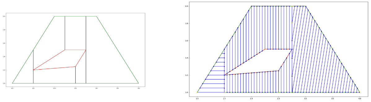
On souhaite générer les points délimitant le boustrophédon de direction optimale sur une surface quelconque, modélisée par un polygone 2D. Le calcul de la direction optimale «theta» de parcours d’un boustrophédon est réalisé à partir d’un algorithme exploitant la propriété convexe d’un polygone pour obtenir un résultat en complexité linéaire sur le nombre de points du polygone (rotating calipers). Une fois cela fait, il suffit d’intersecter le polygone avec des droites parallèles de direction theta espacées d’une largeur de fauchée «d» à définir.

Réunion Teams avec chaque sous-groupe travaillant sur Saturne, pour faire un point sur l’avancée et les besoins futurs qu’ils pourraient avoir (notamment en terme de tests sur le robot réel). Discussion avec Hamid et Robin sur l’organisation des cours.
Recherche d’un algorithme de décomposition d’un polygone en parties convexe. Le choix d’un algorithme de décomposition trapézoïdal avait été fait le séance dernière, car cette forme s’adapte bien aux boustrophédons. Après une seconde recherche pour voir si d’autres solutions convenait mieux au problème, l’algorithme de type «sweep line» est celui qui semble le plus s’adapter au problème.

Implémentation du Sweep Line:
Implémentation du classement de chaque sommet du polygone pour le traitement.
Lecture de la partie expliquant les actions à effectuer pendant le Sweep Line.

La séance d’aujourd’hui a été consacrée au test et au de-bug de l’algorithme de décomposition en parties convexes, ainsi que d’un cas particulier du calcul de direction optimale d’un boustrophédon. Après fusion avec le premier algorithme, qui donnait la direction optimale du boustrophédon sur une partie convexe, on obtient :

où les points jaunes correspondent au départ et à l’arrivée de chaque boustrophédon. Le travail de la prochaine séance sera de déterminer dans quel ordre parcourir les boustrophédons (classe les points jaunes) pour minimiser la distance parcourue non utile. Il faudrait aussi implémenter la fusion des parties convexes adjacentes de même direction de parcours.

The realization of a magnetic map of a terrain is a powerful tool especially used in mine warfare. This cartography can be done with a magnetometer, but the task is quite slow. This is why it is useful to use robots to make this cartography. The problem induced by this solution is the addition of magnetic disturbances related to the structure of the robot and its actuators. It is then possible to drag the magnetometer on a sled behind the robot.

Formalism

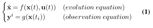
A. Mathematical context. The system evolve on a field which should be mapped with the magnetometer. It follows the evolution describe by EQUATION1.

Where x is the state of the robot, u is the input of the system. As x and u continuously evolve with time, we define the trajectories of this system denoted by x(·) and u(·). We could also define tubes enclosing these trajectories at everytime denoted by ∀t, [x](t) and ∀t, [u](t). Measurements areavailable at each ti and are denoted by yi. Therefore it is assumed that ∀t, u(t)∈[u](t) and that for each measurements yi∈[yi]. This last conditions means that each measurementis bounded which is an assumption made frequently when weare dealing with constrain programming.

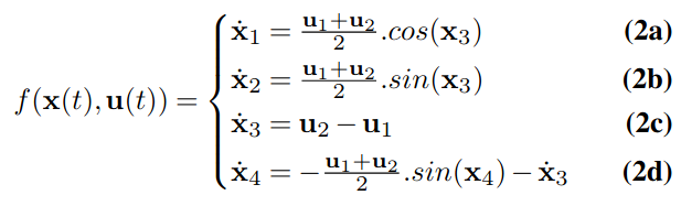
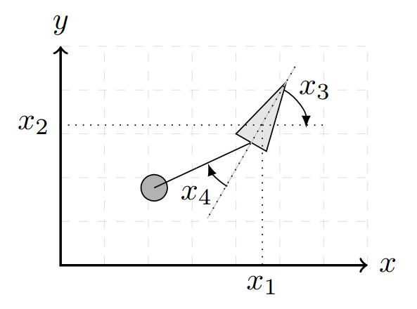
B. State equations. The system is composed of a vehicle that will drag a sledge that transports a magnetometer. The towing vehicle is a tank type vehicle, and the sled is attached to it with a rope. Assuming that the rope is constantly under tension, we are able to find the equations describing the dynamics of the system.

Here x1, x2 and x3 are respectively the abscissa, the ordinate and the heading of the trailing robot, x4 is the angle of the sled to the tractor vehicle, as shown in FIGURE1. We can alsonotice that u1+u2/2 is related to the speed control of the char robot and that u2−u1 is the angular acceleration control.

Constrain Network

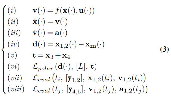
C. Decomposition. These equations could be broken down into the following set of elementary constrains :

These constrains involve intermediate variables introduced for ease of decomposition: tubes v(·)∈R→R4 and a(·)∈R→R2 which are the speed and the acceleration tubes, d(·)∈R→R2 which is the distance between the sled and the robot, t(·)∈R which is the sled angle in the map frame.

Simulator
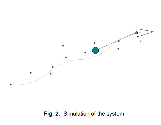
A python simulation was realized using VIBES in order totest the behavior of the system. A class Tank has been cre-ated to instantiate a vehicle with its sled. Then the script in-tegrates the evolution equation using Euler’s method in orderto obtain the state of the systemxaccording to theuinputs.We could see that the behavior of the system seems correctand the model is faithful to reality. Moreover, the GNSS sensor and an accelerometer are simulated in order to enclose the real position in a box.

Reliable set of sled’s angle
Considering that the rope remains continuously under tension while the robot is moving, then the evolution of the angle x of the sled relative to the towing vehicle is described by theDifferential Equation??.

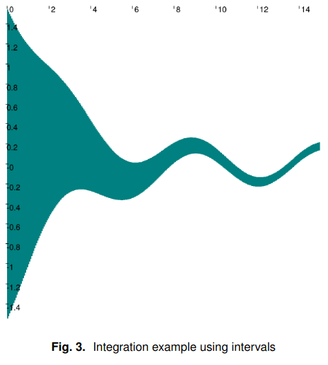
We are able to find the trajectory of the sled by computing the interval containing the angle x4, considering that initially x4 belongs to [−π/2;π/2]. Then by applying the Differential Equation?? on this interval, knowing the control vectoru, we end up obtaining a fine interval framing the real angle x4, independently of the initial angle as we can see on theFIGURE3.

Sled localization
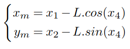
By having a box enclosing the trailing robot, and an interval framing the angle x4, we are able to obtain a box containing the sled, knowing the length of the rope. This box has the shape of a pie sector. Equation4 presents the position of the magnetometer as a function of the state of thesystem x1, x2 and x4. Here all these variables are intervals. By applying a polar contractor to these intervals, we are able to obtain the intervals containing xm and ym.

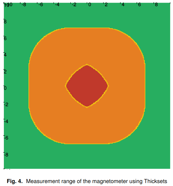
Magnetometer range of measurement

By knowing a box containing the magnetometer and its measuring range, we are able to find all the points seen for sure and all the points that could be seen by the magnetometer. This allows us to recover the coverage of the area by the magnetometer.

Magnetometer Mapping
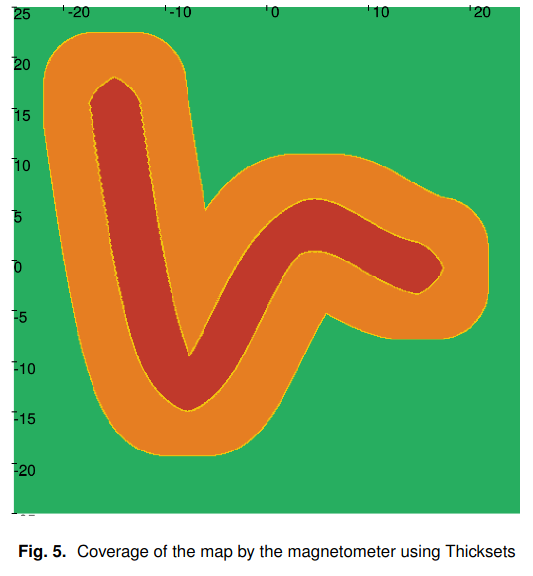
With a moving box enclosing the magnetometer at any time,this method allows us to recover the coverage of the area bythe magnetometer. Thus we have a way to know precisely the coverage of the mapping during the mission, which depends on the uncertainty on the position of the magnetometer and on the maximum distance of each point of the field to be measured. An example of the covered area of a magnetometer ona field is presented by the FIGURE5.

Application example
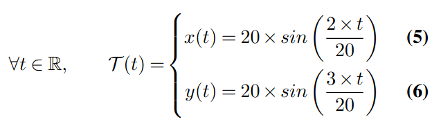
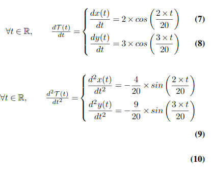
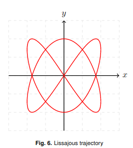
In this part we will see on a practical case what we are able to do with this implementation. We place ourselves in the same conditions as before, i.e. we are in the case of a magnetometer dragged by a robot with tank type evolution equations and the rope must remain tight all along the mission. Here we want our robot to follow the following Lissajous trajectory:

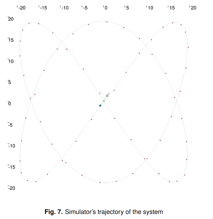
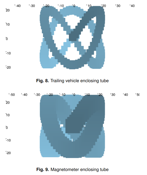
The control.py file is able to generate the controls to drive the trailing robot. These commands are generated by feedback linearization by controlling the robot in speed and heading. These controls leads to the trajectory in the simulator as we could see on the FIGURE7 Then the module mapping.py allows to process the tubes including the trajectory of the trailing robot and the sledge. The tubes are then displayed in order to check that they seem to stick to the trajectory of the system.

Amélioration :
Mise à jour du rapport final au niveau du formalisme du problème. Mise à jour de l’article correspondant.
Préparation de la présentation des travaux réalisés sur un Beamer Latex
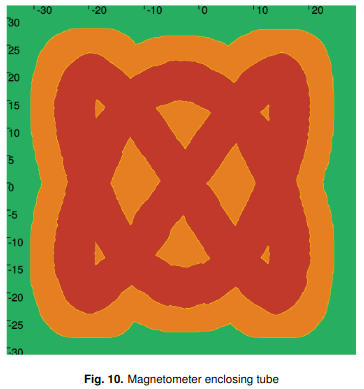
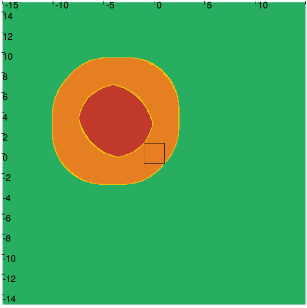
Augmentation de la précision du calcul de la couverture du Magnétomètre à l’aidedes ThickSets appliqués directement à partir du robot tracteur Saturne ce qui nous évite d’introduire un contracteur polaire pour obtenir une boite qui englobe le magnétomètre, mais qui nous introduit beaucoup de pessimisme. On obtient donc le thickset suivant par exemple :

En supposant saturne dans la boite noire [[-1, 1], [-1, 1]], la corde le liant à la luge mesurant 5 mètres et l’angle entre Saturne et le magnétomètre étant comprise entre3pi/4 et 4pi/5, on obtient les zones visibles à l’écran avec la zone rouge qui est vue à coup sûr et la zone orange qui est peut-être vue avec un distance de détection de 5mètres ici. On remarque que la forme est similaire au Thickset que l’on avait déjà puvoir auparavant, mais avec la méthode précédente on obtient un Thickset inclu dans celui-ci dans la mesure où la zone rouge se trouvait à l’intérieur de la nouvelle zone rouge, et la zone orange était bien plus grande.
On obtient donc des résultats bien plus intéressants qui permettent de montrer la puissance de cette méthode d’estimation de l’angle. Pour rappel, on est ici capable de trouver la zone vue par le magnétomètre uniquement grâce à un GPS dans le robot tracteur et sans ajout de capteur mesurant l’angle de la corde.

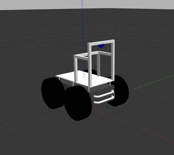
Avancement dans la simulation Gazebo, le modèle du robot s’affiche correctement dans gazebo et les roues tournent avec des commandes ROS. Cependant les roues tournent mais le robot n’avance pas. J’ai essayé de modifier les coefficients de frottements des roues sur le sol mais le problème ne vient pas de là. Il semble que le robot est fixe, même en appliquant des forces je ne peux pas le bouger.

Dans le cadre de la prise en main du robot Saturne nous avons fait la mise en service du robot et nous avons testé les codes existants. De plus nous avons commencé à adapter les codes de Saturne afin de pouvoir charger une mission quelconque à partir d'un fichier. Le fichier devra comporter ligne par ligne les étapes de la mission. Le format exact du fichier de mission reste à déterminer et pourra éventuellement être adapté au besoin des autres groupes. Durant les prochaines séances nous devrons tester les codes adaptés sur le vrai robot et enregistrer les données de localisation du robot et de la luge pour le groupe qui travaille sur la localisation de la luge.

Nous avons effectué la configuration du GPS de Saturne pour qu’il puisse recevoir les corrections RTK. Ensuite nous avons adapté les codes du serveur pour que les corrections RTK soient envoyés vers deux GPS mobiles. C’est-à-dire que le serveur accepte deux connections TCP.

Un premier test grandeur nature a pu etre effectué et un time lapse à été effectué

De nouveaux tests sur terrain ont été effectués, le tout filmé avec un drone